


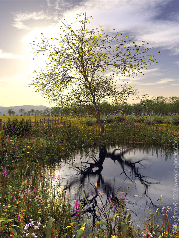
Artwork created in 2002
Modeling and rendering natural landscapes featuring thousands of plants require important computer resources. In POV-Ray, plants built with Constructive Solid Geometry are useless for making large vegetal covers such as forests because they are too memory-consuming, and it is normally more efficient to use meshes instead and to copy them over and over to benefit from mesh instantiation (unlike CSG objects, meshes can be replicated with little memory overhead). Since there are few free or cheap plant mesh generators (like Arboretum or Gena Obukhov's graphic version of Tomtree), POV-Ray users rarely do large "green" landscapes. There are several commercial products though, and in March 2002, Greenworks, the maker of Xfrog, a modeler specialising in the creation of complex organic structures, asked me whether I?d be interested in using it. In the next months I made 6 images containing Xfrog plants (Winter, In vitro, The prince, Not for sale anymore, The accident and Persistence) to be featured on the Greenworks website. Still, I had barely explored Xfrog's modeling capabilities, having only used pre-made Xfrog models or created imaginary plants. It was time to do a little more complex, the landscape equivalent of the city images that can be see on this website, and to create original models based on real plants. I quickly came up with a simple idea ? a backlit tree, a pond, and the ominous, mismatched reflection of the tree ? and started working.
The first challenge was the main tree, because it was backlit and the light was supposed to shine through. POV-Ray can do "double illumination" which allows for the side of a surface opposite to a light source to be illuminated like the one facing it. However, the effect cannot be really be controlled: the opposite side is as illuminated as the side facing light, which is not realistic. I ended up using this feature for the smaller plants, but for the tree I did it the hard way, using scattering media to simulate the leaf material. The original tree was a Japanese maple, chosen to be large enough without being too dense. In Xfrog, its leaves are little squares textured with a half-transparent picture of the real leaf: they are beautiful, but unfit to be used with scattering media as they are mathematically flat. For this reason, I replaced them by a proper media container, consisting of an Xfrog "horn" component shaped and flattened like a simple pointy leaf but with a real "inside". The leaves were not as nice as the original maple ones (this would have been too costly in terms of polygon count), but they were now behaving like true leaves.
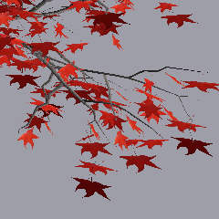 | 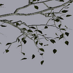 | 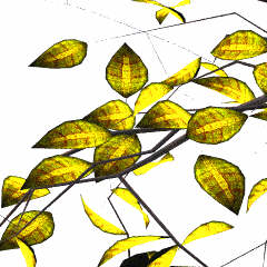 |
| Original leaves (flat polygons) Xfrog render | Modified leaves (flattened "horns") | Modified leaves backlit POV-Ray render |
We can see in the third picture that the texture of the final leaves isn't still too great, and also that the leaves have a low resolution due to the efforts needed to keep the total polygon count as manageable as possible. The entire tree has still 500000 polygons and "weighs" about 70 Mb? Because of this, tweaking the media took a long time and there are some unsolved artefacts.
The tree in the reflection was much easier to do, being an imaginary species, right from "Sleepy Hollow". Here is a screenshot of the model within Xfrog.
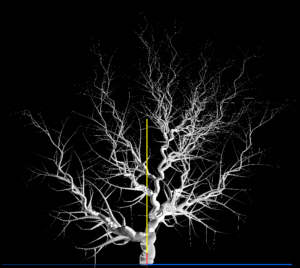
With the main trees was more or less secured, I started working on the other plants. For the background, it was enough to recycle a pistacia bush, a cherry tree and few token weeds from the previous Xfrog images. The foreground species were selected in an old flora (European wild plants, by Björn Ursing, 1955) so that they would be plausible in a pond environment, visually attractive and not too hard to model for a beginner. The Xfrog screenshots for these species are shown below:

Several models of these plants (different sizes, flowering stages and number of leaves) were created.
One of the most important and complex feature of Xfrog is the ability to use customised mathematical functions to control the shape of the plant components. For instance, the "break" on the reed leaves was obtained by the following expression, that returns the leaf curvature (in degrees) as a function of the position x (between 0 and 1) on the leaf: (1-floor(x+0.44))*floor(x+0.46)*-100. This function returns 0 (= no curvature) for most of the leaf, but returns -100 degrees for the segment comprised between 54% and 57% of the relative length, causing the leaf to break suddenly a little after its midpoint. POV-Ray users with some coding experience won?t find this very difficult... It's a lot of fun actually and quite simple, at least if one doesn't aim for a total botanical accuracy.
The last problem was the textures: since I couldn?t really collect these plants in their natural environments, I just scanned some similar-looking leaves from the garden at my workplace, and modified them in Picture Publisher. Other textures were recycled from the Xfrog libraries.
A common problem with TGA, PNG and TIFF maps containing alpha (transparent) channels, such as the ones typically used for leaves, is that a texture made with such a map has the same finish properties for both the transparent and non-transparent areas, so that highlights and reflections typically show up on the transparent ones, revealing the underlying shape as if it was actually made of glass. For instance, a leaf will look like a bright square or triangle because the transparent part also reflects light when it should be empty. To fix this requires using an image_pattern created as follows.


Here is a typical declaration for a leaf texture using the leaf mask and the leaf pigment maps above:
texture{


image_pattern{jpeg "leaf_mask"} // used for the transparency


texture_map{


[0 pigment{Clear}finish{ambient 0 diffuse 0}]


[1 pigment{image_map{jpeg "leaf_pigment"}} finish{ambient 0 diffuse 1}]


}

}
The last touch was to add double illumination to the petals, in order to create the backlit effect there too.
Creating realistic skies in POV-Ray alone has many advantages but requires a lot of tweaking, and, if media is used for clouds and other atmospheric effects, the render times can become unbearable for large images. For this reason, I have used Terragen-made background for most of the recent landscapes, as Terragen can produce beautiful skies and clouds, quite recognisable but nice enough for most purposes. Terragen's image output has (almost) no size limit and can be as large as the image where it will be used, hence reducing the risk of having pixels showing up. Photos of real skies would be better, but very large digital photos are not very common (or they are expensive).
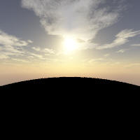
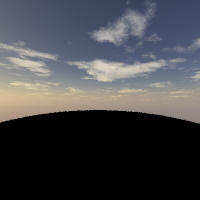
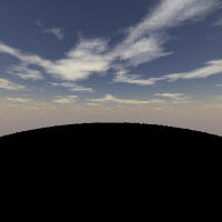
Terragen cannot produce directly a sky dome, so the usual technique is to create a panorama made of five panes: front, back, left, right and top. To get a seamless panorama, the easiest is to have a viewing angle of 90° (set the Zoom/Magnification parameter at 1). If the image is square, the panorama will be perfectly seamless. If the ratio is different, only the front, right, left and back will be seamless. Then set the camera parameters as follows in sequential order:
This can be automated using Terragen?s scripting feature. If you?re doing animation and if you need a complete panorama where all the panes have the same resolution, this is probably the best solution. In the case of large POV-Ray images, only the visible pane needs to be rendered at full resolution: the other panes just contribute to the global illumination so they don?t need a high resolution. The Terragen render can also be quicker if the landscape is turned off (the bottom part will appear black).
A typical Terragen panorama looks like this in POV-Ray code:
#declare Panoramic=union{

    object{Pane texture{pigment{ image_map{jpeg "sky_front"}}
finish{ambient 1 diffuse 0}}}

    object{Pane texture{pigment{image_map{jpeg "sky_right"}}
finish{ambient 1 diffuse 0}} rotate y*90 translate x}


    object{Pane texture{pigment{image_map{jpeg "sky_back"}}
finish{ambient 1 diffuse 0}} rotate y*180 translate x-z}

    object{Pane texture{pigment{image_map{jpeg "sky_left"}}
finish{ambient 1 diffuse 0}} rotate y*270 translate -z}

    object{Pane texture{pigment{image_map{jpeg "sky_top"}}
finish{ambient 1 diffuse 0}} rotate -x*90 translate y}

    translate z*0.5-x*0.5-y*0.35 // centers the panorama around
the origin and lowers it at horizon level


    scale 1500 // size of the panorama box

    no_shadow // so that a light source can be positioned outside
the sky box

}
 |
Here are the 5 sky maps in low resolution. |
 |
  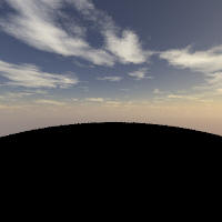 |
The water was just a plane and the only sophisticated feature was the small ripples of different sizes:
#declare colWater=rgb <78,104,48>/255;

#declare matWater = material{


texture {


pigment{rgbt}


normal{


pigment_pattern{


bozo


color_map{


[0.45 Black]


[0.55 White]


}


}


normal_map{


[0 waves frequency 400 bump_size 0.01 turbulence 0.1]


[1


function {


f_noise3d( x*1, y*5, z*5)*0.8


+f_noise3d( x*10, y*50, z*50)*0.2


+f_noise3d( x*100, y*200, z*200)*0.2


}


bump_size 0.004


]


}


}


finish {


ambient 0


diffuse 0.2


specular 1


roughness 1/500


metallic


brilliance 2


reflection {


0.6,1


fresnel on


}


conserve_energy


}


}


interior {


ior 1.33


}

}
The terrain is just a 1024 x 1024 height field painted with Picture Publisher, replicated by seamless tiling across the entire landscape.
The hills visible near the horizon are actually part of the Terragen landscape.
The lighting is made up of two light sources: one is the regular sun and one is a bluish light coming from above (the radiosity needed a little help?).
However, there is also a big cheat?While the ?official? sun position was all right for the scene, it didn?t shed enough light on the tree itself, which was poorly illuminated. To get some visible sun on the branches, I gave the tree its own local sun coming from a position situated at 25° on the left of the official position. Let's call this poetic license...
Radiosity is used, with extremely low settings (count 10, error_bound 1) that are suitable for this sort of image (many small objects, many different textures).
The dragonflies (made in Rhino) and their twigs (isosurfaces) were recycled from The lovers. The frog is a standard Poser one. All those animals are hardly visible at screen resolution and they are some sort of Easter eggs for the people who will buy the poster!
Now that all the elements of the scenes were ready, the last task was to plant thousands of copies of the 27 different plants. This sort of work just requires some patience, because a lot of tweaking is necessary and plant models take a long time to parse. One way to handle massive quantities of objects is to store them in arrays. In this case, there are 5 of them:
Several loops take care of the positioning. The main one is a big loop of 12000 plants that put the "reeds" just above or just below the waterline, the "grasses" everywhere else and the "nettles" in one tight spot. Each plant has a dummy counterpart and flags are used in the code to switch between the dummies and the final models, to save time during the testing.
Here is the main loop for the "reeds", "grasses" and "nettles". Other loops put the ?floaters? and the ?trees? where they belong.
#declare rd=seed(125);

#while (i
    #declare Norm=<0,0,0>;


    #declare aPlant=35+145*rand(rd);

    #declare Start =
vaxis_rotate(<0,5,-1+rand(rd)*0.7>,y,aPlant)+x;

    #declare Pos= trace ( Terrain, Start, -y, Norm ); // uses
trace to put the plant at the right height

    #if (vlength(Norm)!=0)

        #if (Pos.y<-0.5+rand(rd)*0.4) //
close to the waterline


            #declare
Plant=object{Reed[int(nReed*rand(rd))] scale (0.5+rand(rd)*0.5)}

        #else // elsewhere

            #if
(vlength(<0.2,Pos.y,0.2>-Pos)>0.06) // nettle location


#declare Plant=object{Grass[int(nGrass*rand(rd))] scale
0.3+0.95*abs(cos(5*(aPlant-45)*pi/180))}

            #else


            #declare
Plant=Nettle[int(3*rand(rd))]

        #end

    #end

    object{

        Plant

        rotate x*(0.5-rand(rd))*10


        rotate 360*rand(rd)*y

        scale 0.6+rand(rd)*1.7

        scale


        translate Pos

    }

    #declare i=i+1;


#end
Approximately 370 millions of polygons are present in this image. In spite of the radiosity and the area lights, it rendered rather quickly at 6000 x 8000, in a couple of days.
Interestingly, many people miss the discrepancy between the tree and its reflection. The image has been (perhaps rightfully) criticised for this, but I still like the idea that something so "right in your face" can be overlooked so easily.
This image, and several of my first Xfrog ones, is featured in Oliver Deussen's book "Computer-generierte Pflanzen" (Springer-Verlag, 2003).